
Example Notebooks
The repository consists of a collection of self-contained Jupyter notebooks that reproduce the analyses and figures presented in the associated publication. Each notebook focuses on a specific aspect of the evaluation, including spatial climatologies, precipitation statistics, annual and diurnal cycles, sea-surface temperature, and vertical temperature profile analyses.
Each section below provides a brief description of the corresponding notebook together with an example of the generated figure.
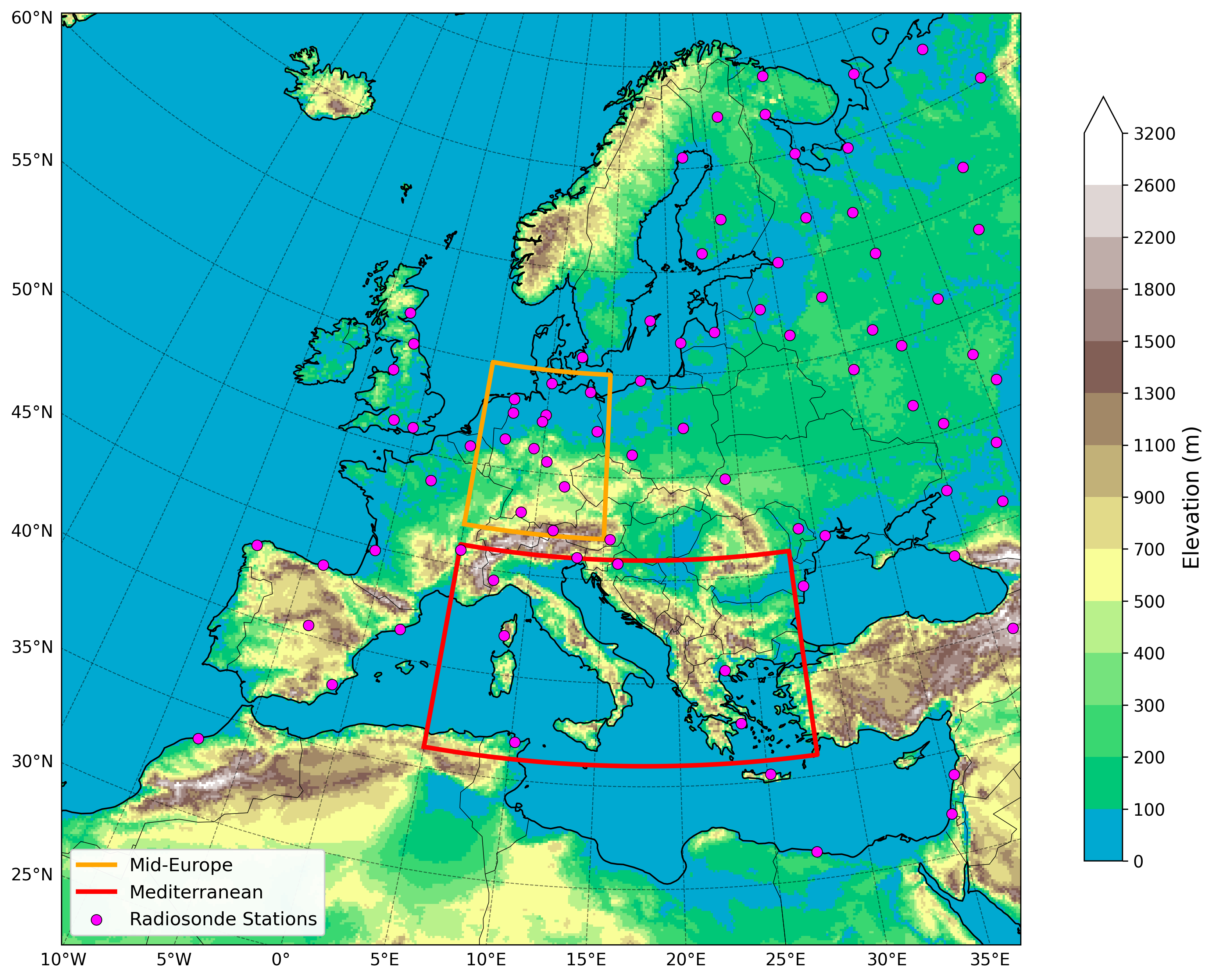
01_domain.ipynb
Description: Visualizes the ICON-CLM model domains used throughout the study.
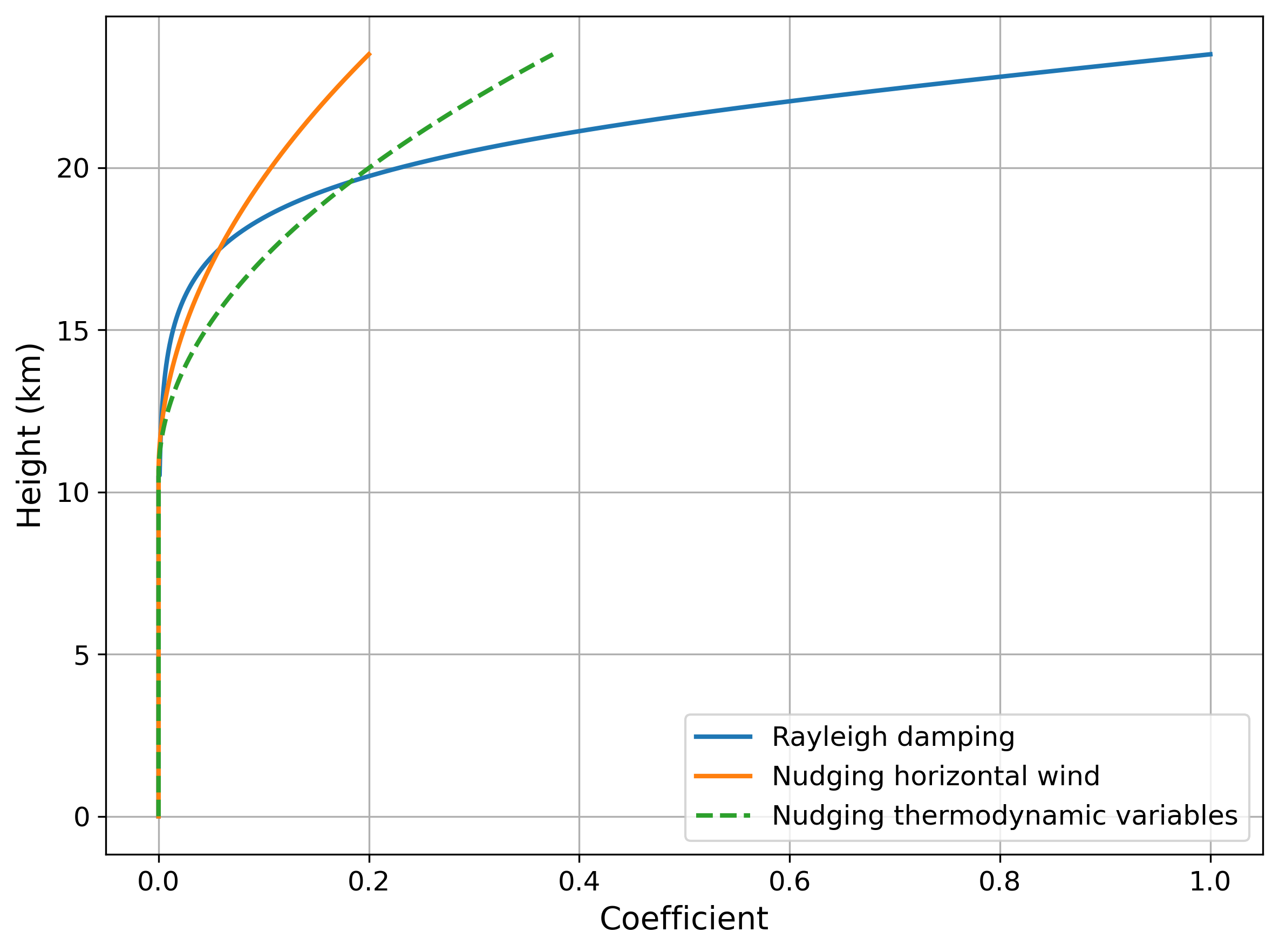
02_upper_boundary_coefficients.ipynb
Description: Compare ICON upper boundary coefficients.
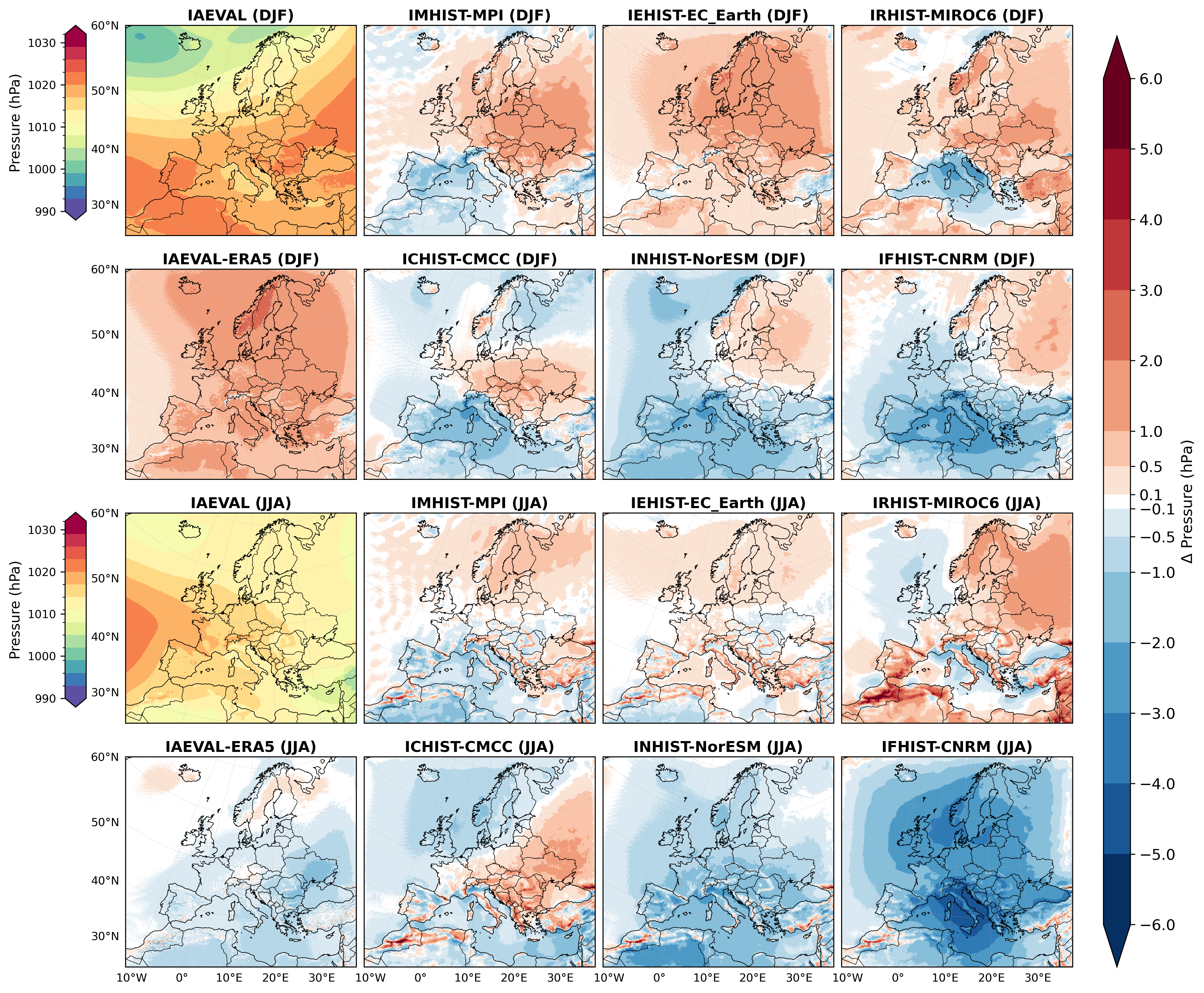
03_PSL_RCM_GCM.ipynb
Description: Compares seasonal mean sea-level pressure fields between RCM and GCM simulations.
04_TAS_RCM_GCM.ipynb
Description: Evaluates seasonal near-surface air temperature differences between RCM and GCM simulations.
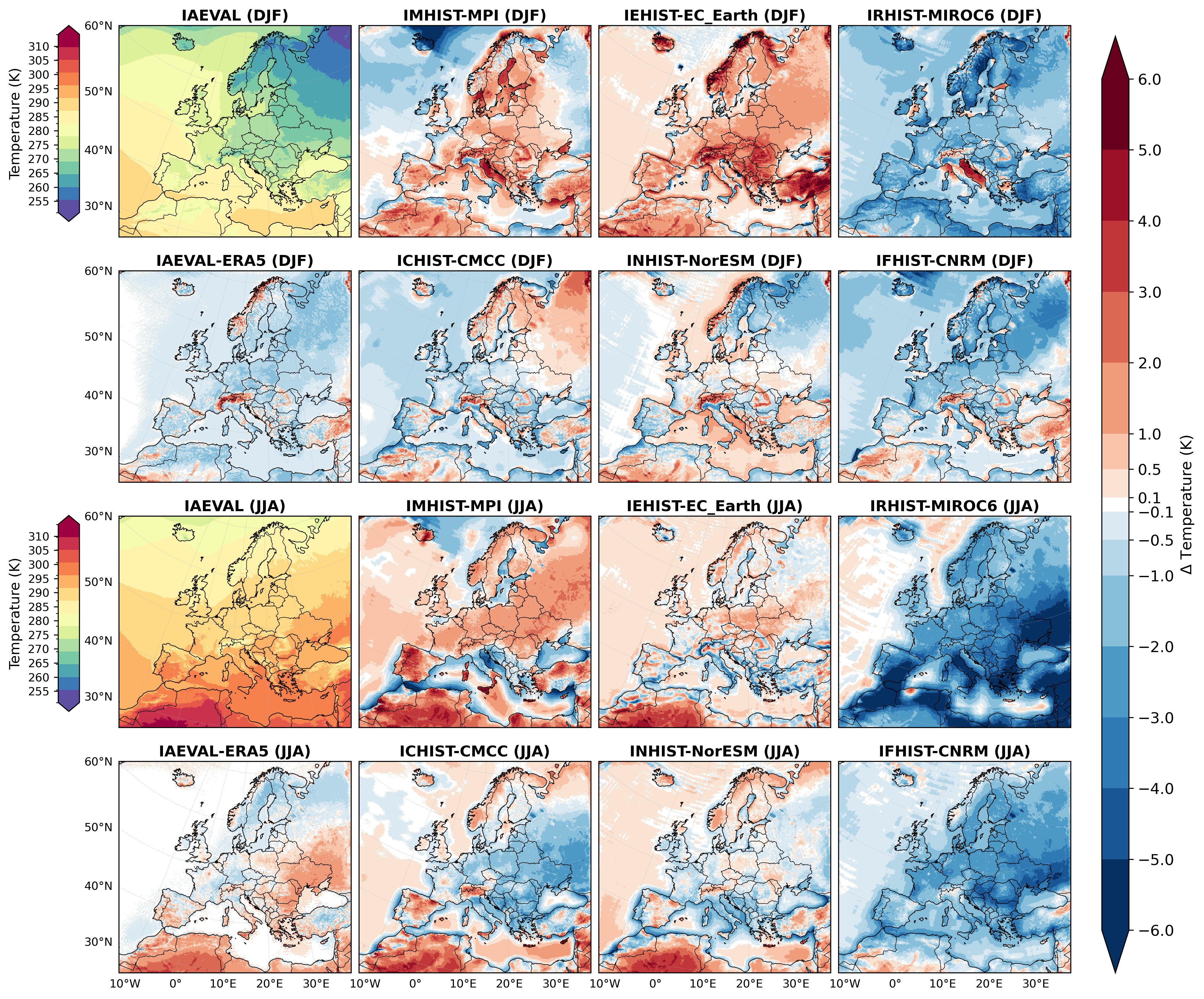
05_PR_Relative_RCM_GCM.ipynb
Description: Shows the relative precipitation differences between RCM and GCM simulations.
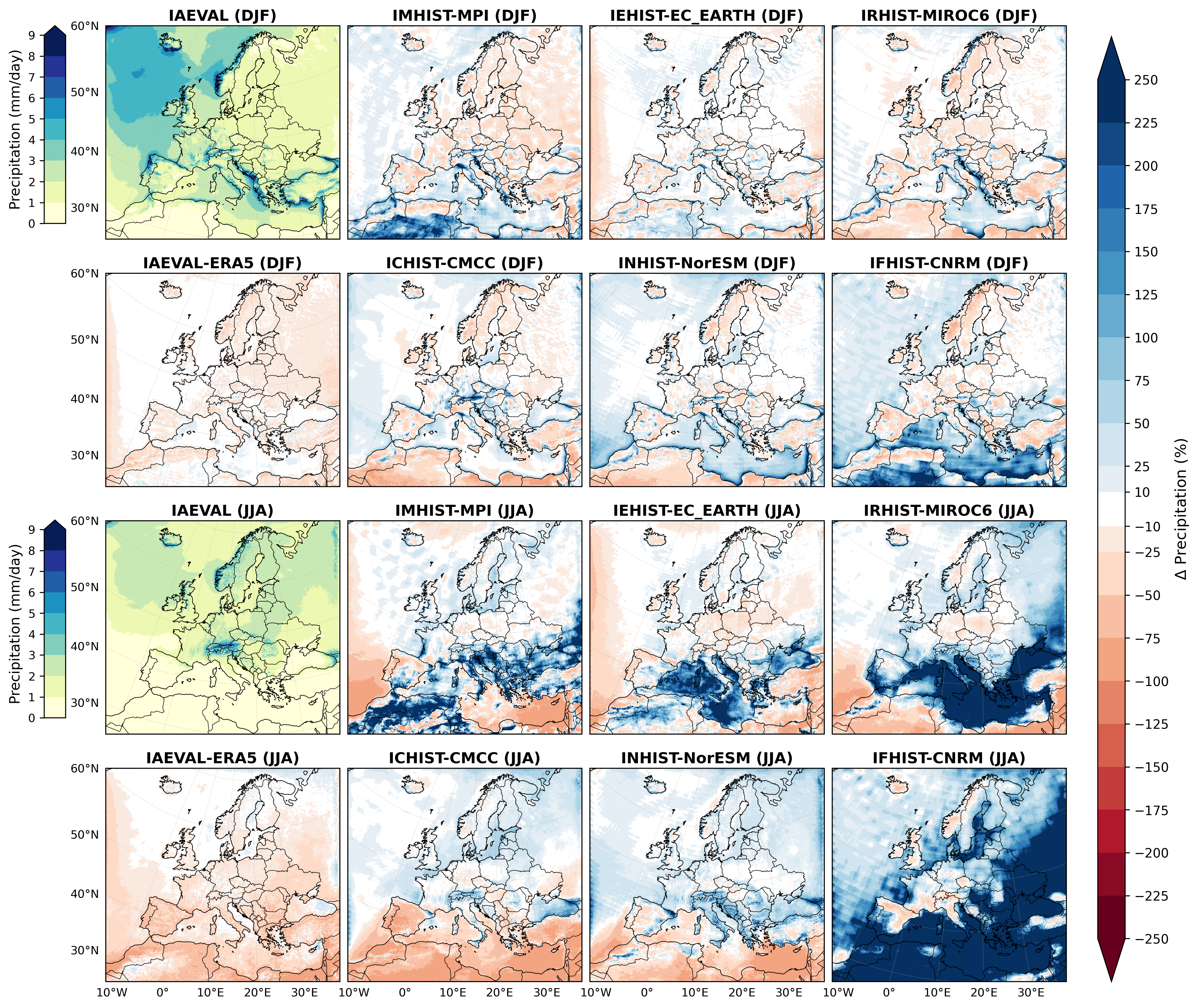
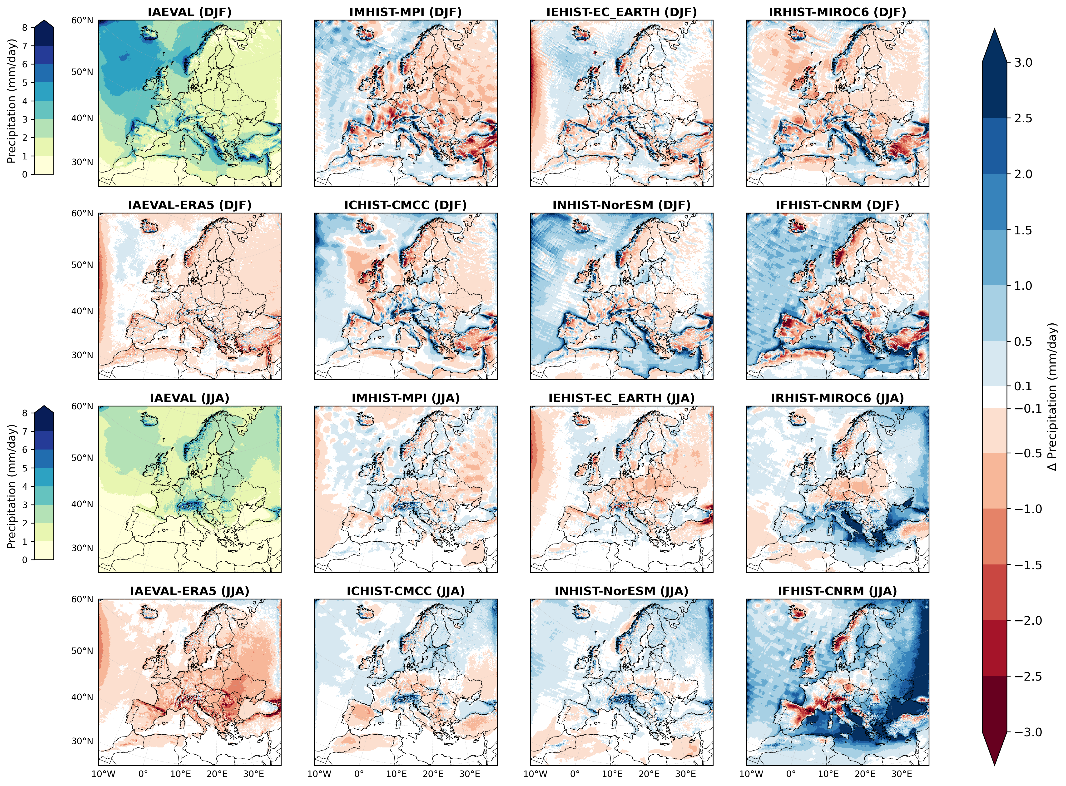
06_PR_abs_RCM_GCM.ipynb
Description: Displays absolute precipitation climatologies together with RCM–GCM precipitation differences.
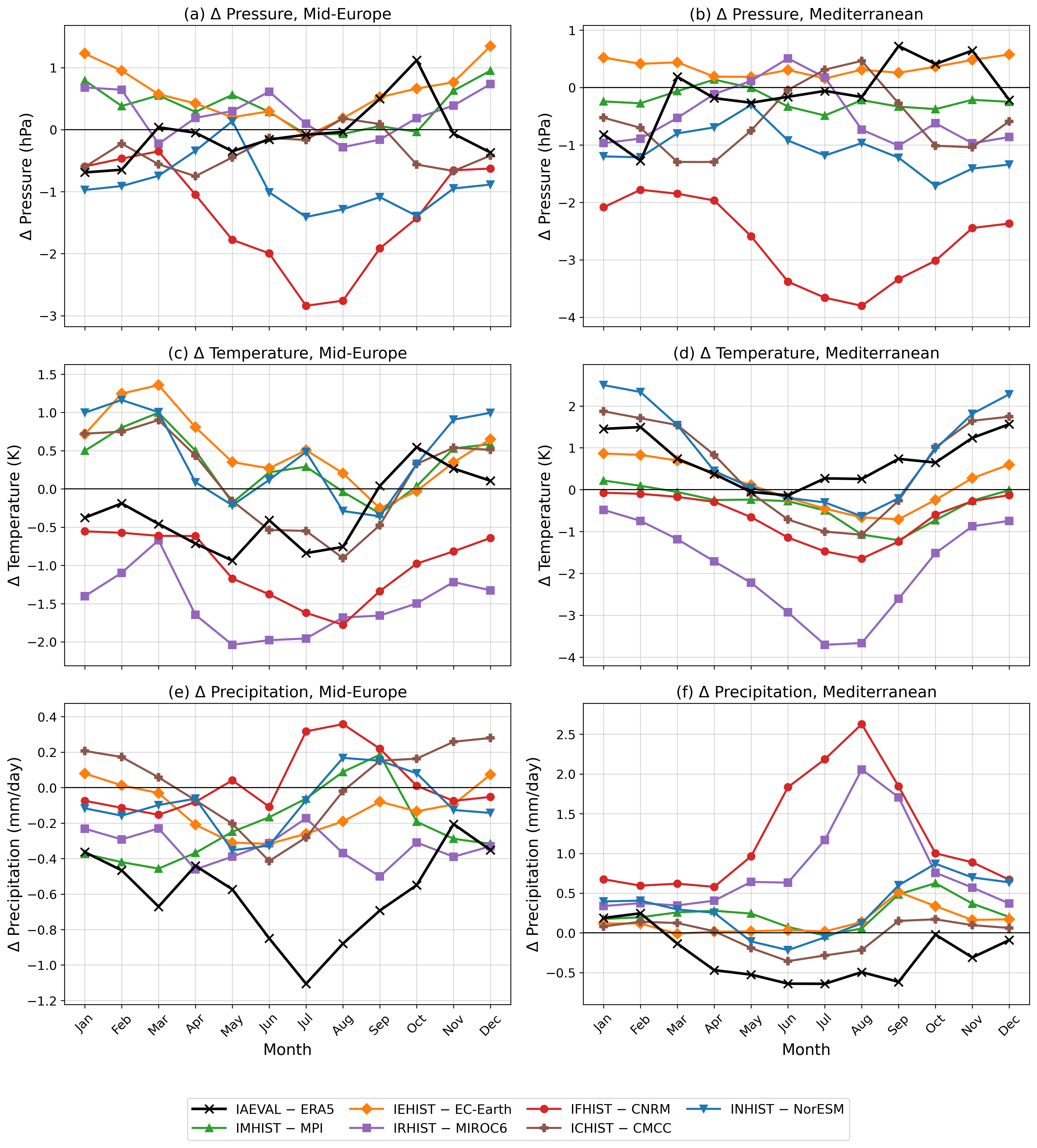
07_annual_cycle.ipynb
Description: Analyzes the annual precipitation cycle over the selected evaluation regions.
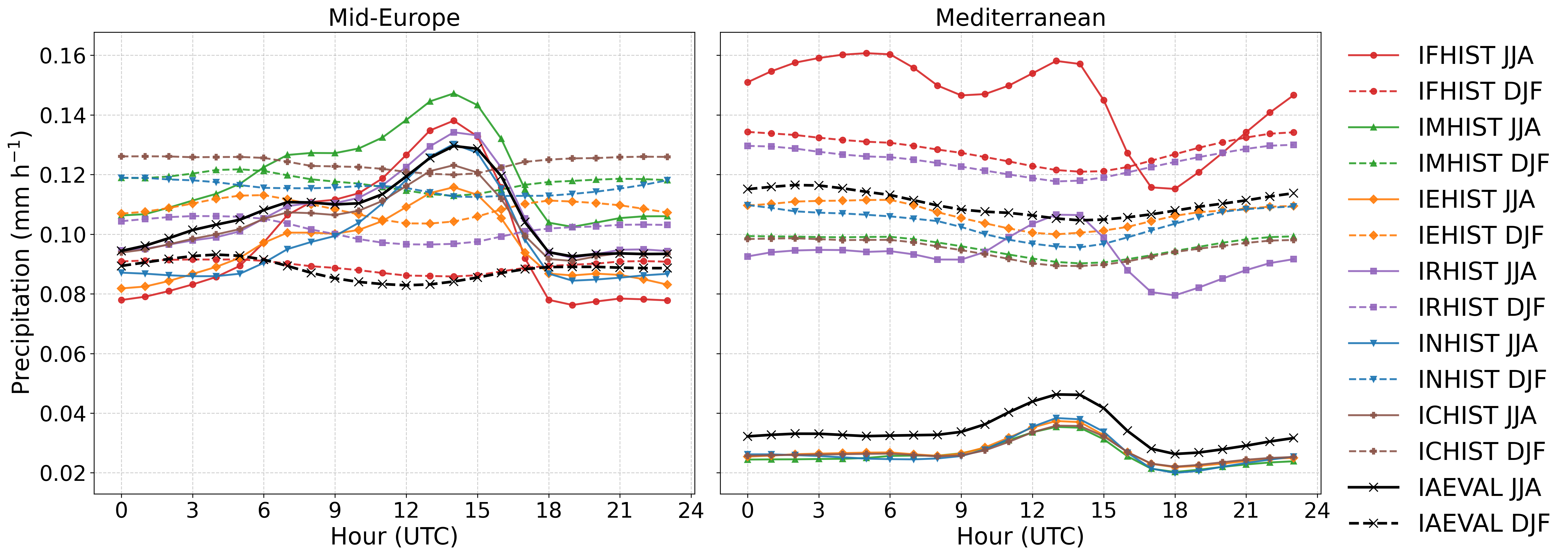
08_diurnal_cycle.ipynb
Description: Evaluates the mean diurnal precipitation cycle across the study domains.
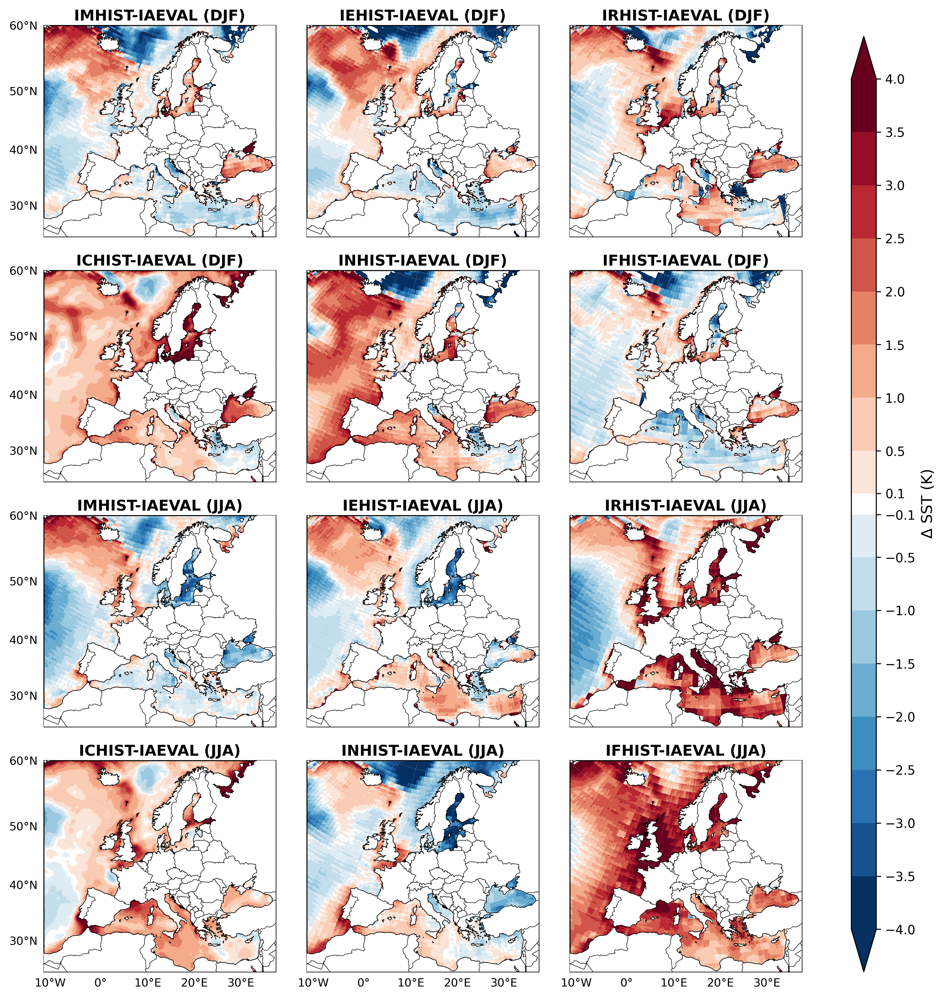
09_SST_RCM_IAEVAL.ipynb
Description: Evaluates seasonal sea-surface temperature differences relative to the reference dataset.
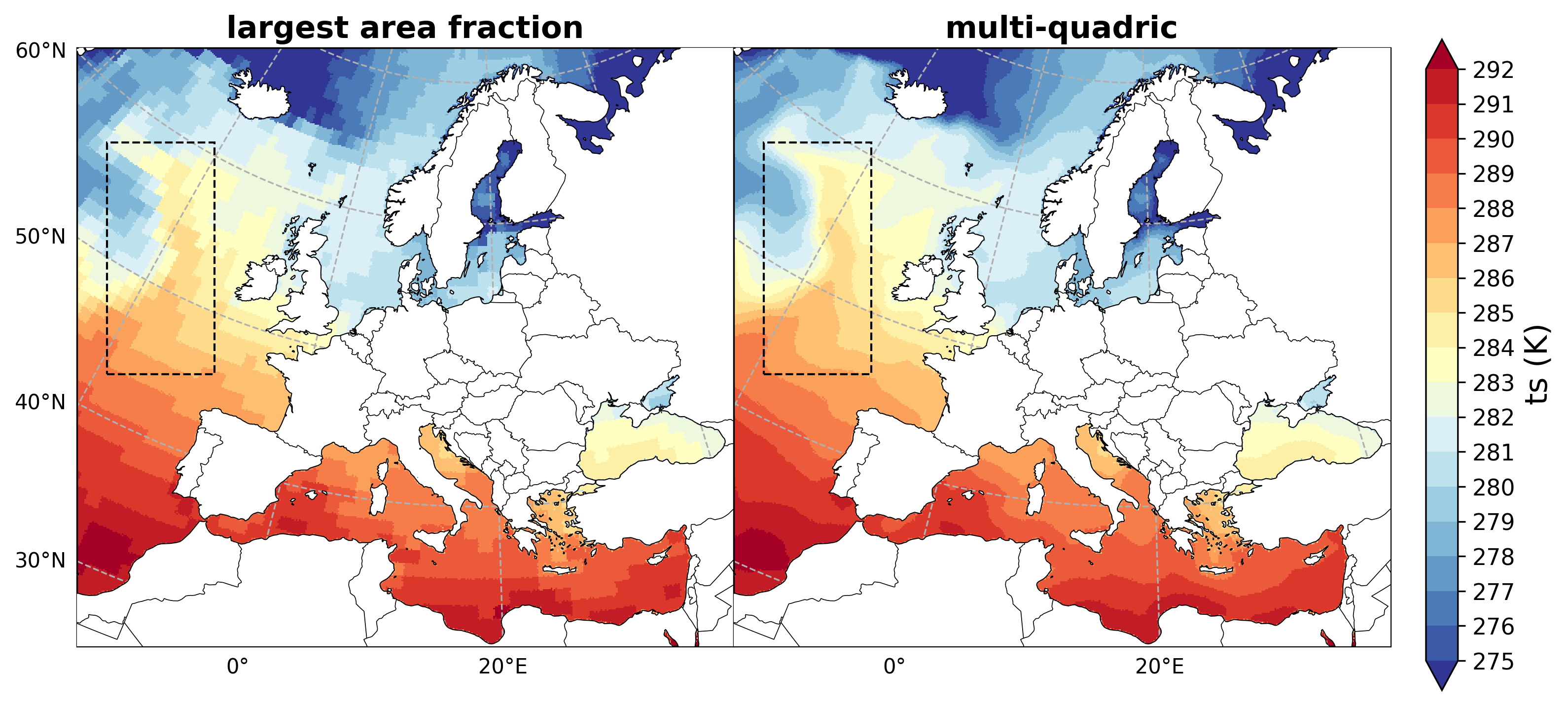
10_SST_interpolation_comparison.ipynb
Description: Compares sea-surface temperatures produced with the two SST interpolation methods and shows their distributions over the selected subdomain.
| Figure 10a | Figure 10b |
|---|---|
 |
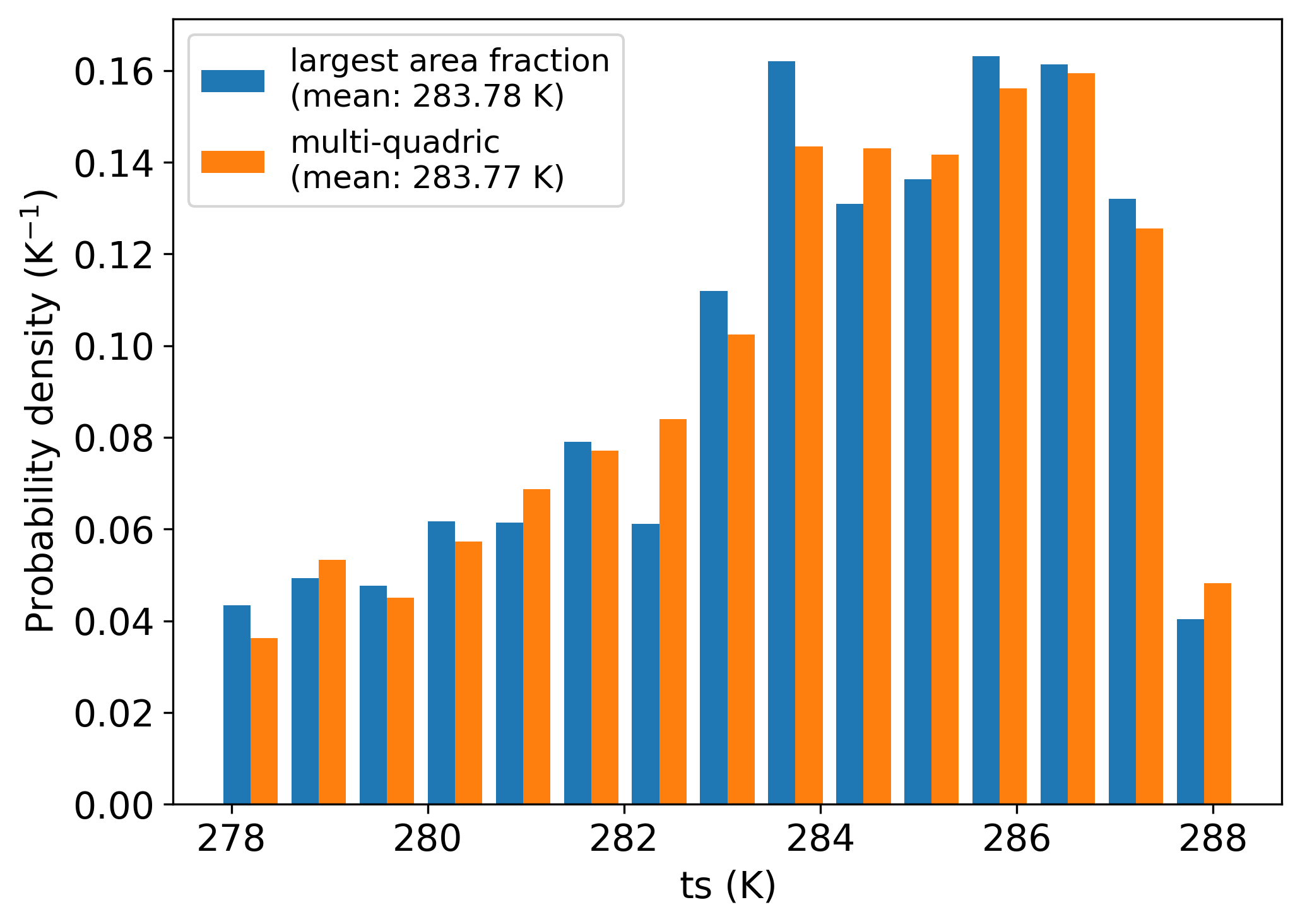 |
| Spatial SST fields | SST distributions |
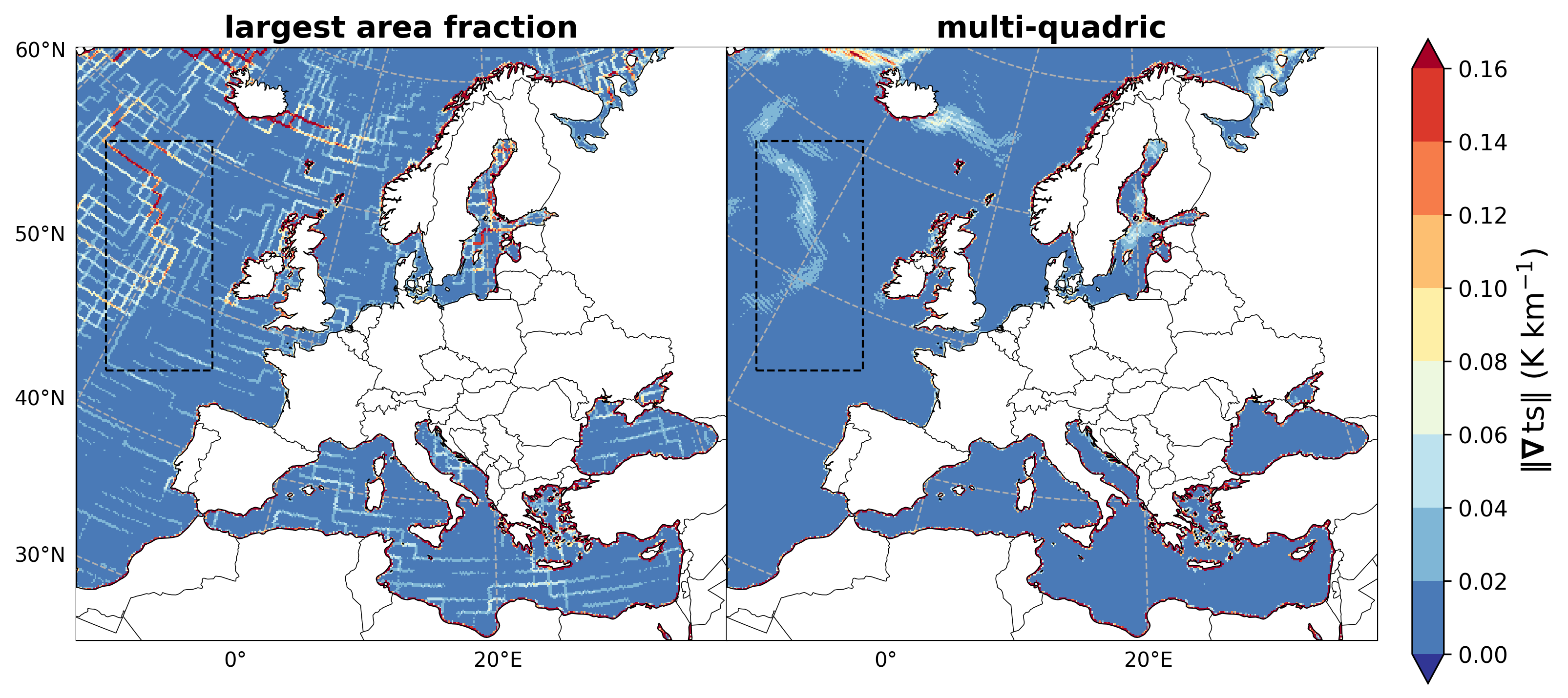
11_SST_gradient_comparison.ipynb
Description: Compares horizontal sea-surface temperature gradient magnitudes calculated from the two SST interpolation experiments.
| Figure 11a | Figure 11b |
|---|---|
 |
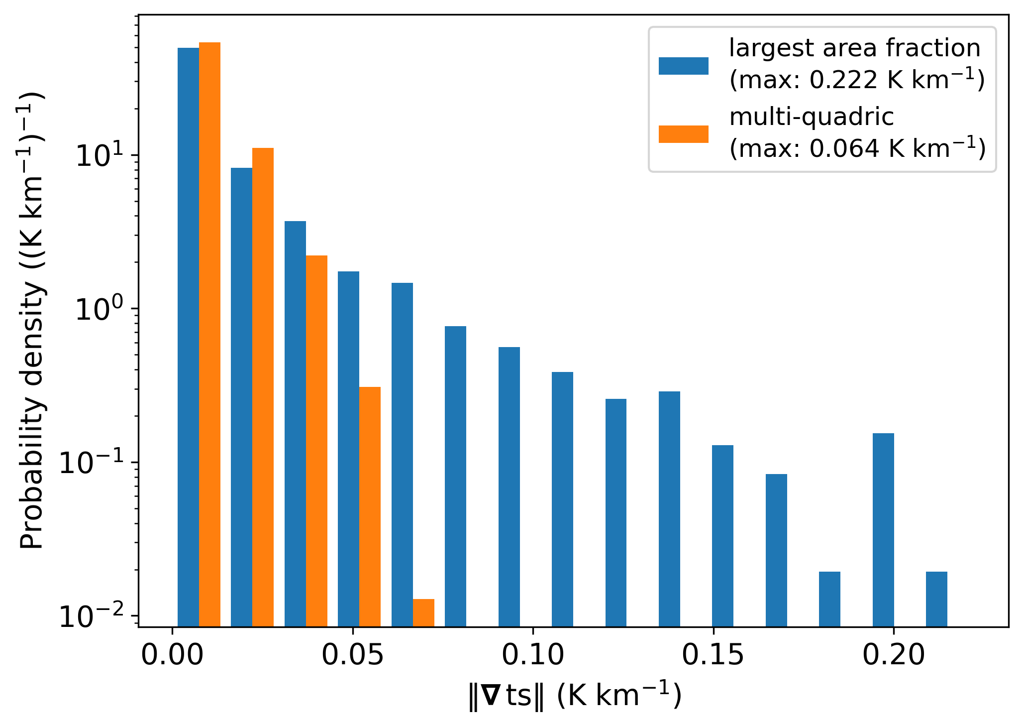 |
| Spatial SST-gradient fields | SST-gradient distributions |
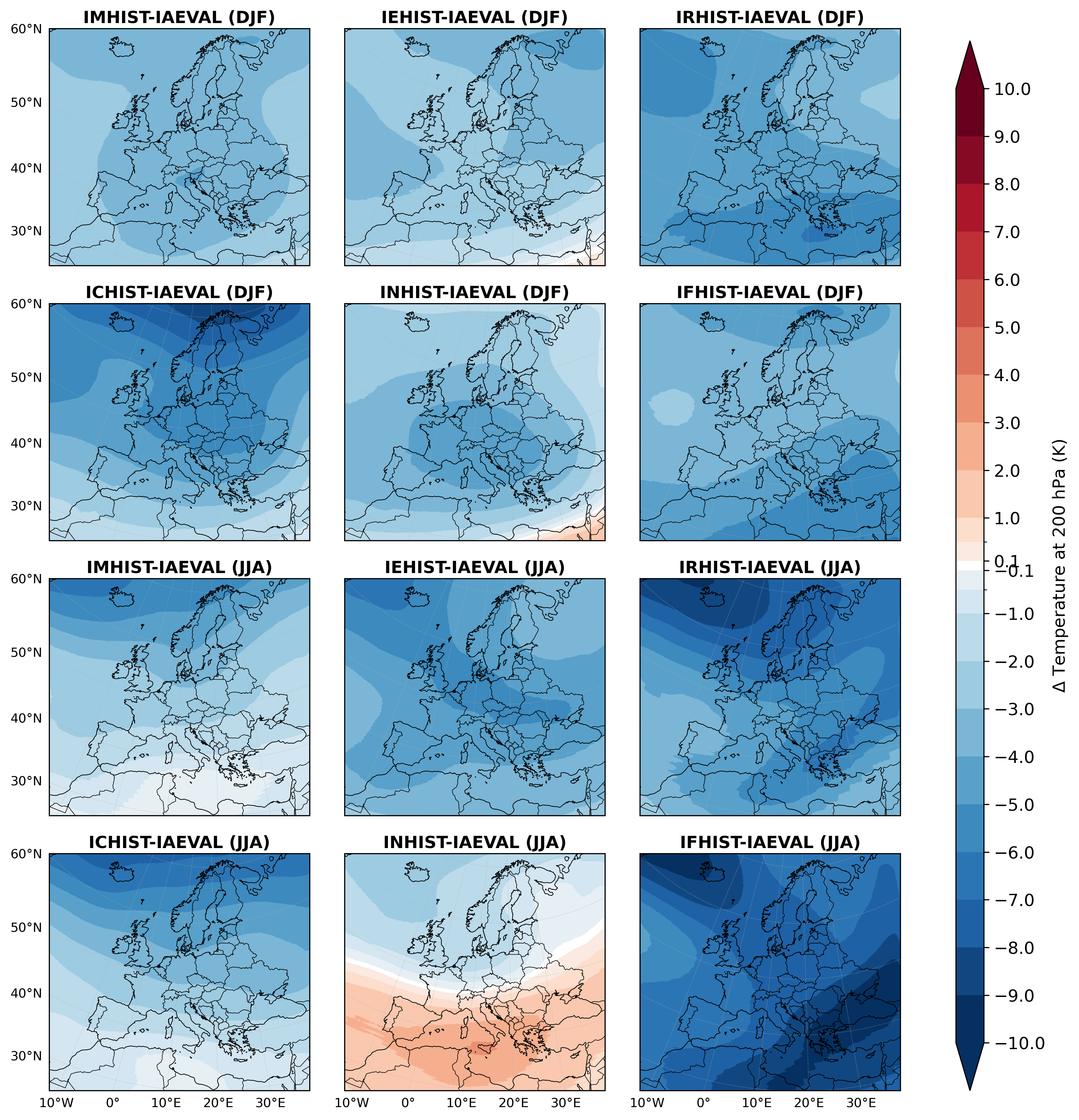
12_T200_RCM_IAEVAL.ipynb
Description: Compares seasonal temperature fields at 200 hPa between simulations and the reference dataset.

13_14_13_14_Vert_TA_domains.ipynb
| Figure 13 | Figure 14 |
|---|---|
 |
 |
| Spatial SST-gradient fields | SST-gradient distributions |
15_Vert_TA_profile_MID_EU.ipynb
Description: Displays seasonal vertical temperature profiles over the Mid-Europe domain.

16_Vert_TA_profile_MED.ipynb
Description: Displays seasonal vertical temperature profiles over the Mediterranean domain.

17_Vert_TA_gradients_MID_EU.ipynb
Description: Evaluates vertical temperature gradients (lapse rates) over the Mid-Europe domain.

18_Vert_TA_gradient_MED.ipynb
Description: Evaluates vertical temperature gradients (lapse rates) over the Mediterranean domain.